Stratos Hyperscale Data Center
Subsurface Thermal Risk Analysis
Wonder Valley, Box Elder County, Utah — Substrata runs the subsurface physics on the proposed 9 GW Stratos facility: soil conductivity 2.5–7× below standard assumptions, thermal plume crosses water table in every scenario, compounding with documented liquefaction risk on an active fault zone.
1. Site Dossier
The Stratos Project occupies a 40,000+ acre parcel in Hansel Valley, a closed graben within the Basin and Range physiographic province of northwestern Utah. The basin is hydrologically closed, tributary to the Great Salt Lake, with no perennial surface water. The facility is proposed to reach 9 GW IT at full buildout with 16 GW total thermal rejection.
1.1 Key Parameters
| Parameter | Value | Source | Confidence |
|---|---|---|---|
| Valley floor elevation | 1,300–1,340 m | Stratos.md | LOW |
| Mean annual precipitation | < 28 cm/yr | Stratos.md | LOW |
| PET (estimated) | ~120 cm/yr — permanent deficit | Basin-and-Range lit. | MEDIUM |
| Mean annual temperature | ~12°C (estimated) | Derived T_max/T_min | MEDIUM |
| Summer high / winter low | 32.2°C / −7.2°C | Stratos.md | LOW |
| Dominant lithology | Quaternary lacustrine silt/clay | Stratos.md + USGS | LOW |
| Water table depth | ~20 m (est.) | Regional inference | HIGH |
| Vadose zone S_r | 0.10–0.25 (very dry) | Campbell VG from MAP/PET | MEDIUM |
| Geothermal gradient | 35–50°C/km | Basin-and-Range lit. | MEDIUM |
| Darcy velocity (mid) | ~5×10⁻⁸ m/s | Regional estimate | HIGH |
| Fault | Hansel Valley Fault, 22 km trace | USGS fault catalog | LOW |
| Fault slip rate | < 0.2 mm/yr | USGS fault catalog | LOW |
| Liquefaction documented | Yes — 1934 M6.6 event | USGS / Stratos.md | LOW |
| Phase I cap / full / buildout | 1.5 GW / 3 GW / 9 GW IT | Stratos.md | LOW |
| Total thermal rejection (9 GW) | 16 GW | Stratos.md | LOW |
| Cooling type | Closed-loop hydronic + air-cooled dry HX | Stratos.md | LOW |
| Water rights portfolio | 14,900 AF total | Stratos.md | LOW |
Confidence ratings indicate data quality: HIGH = directly measured/stated; MEDIUM = inferred/regional estimate; LOW = unknown/modeled.
1.2 Johansen Profile — Hansel Valley Nominal Stratigraphy
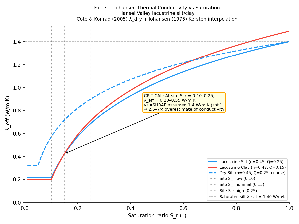
The basin floor is underlain by late Quaternary lacustrine deposits from three major lake cycles (Little Valley ~140 ka, Hansel Valley ~80 ka, Lake Bonneville 30–10 ka). The Bonneville cycle dominates the basin floor surface. Because MAP < 28 cm/yr with PET ~120 cm/yr, the vadose zone above the water table is in a state of permanent moisture deficit. This is the physics-critical site condition — it controls thermal conductivity.
| Layer | Depth (m) | Litho | S_r | λ_dry (W/m·K) | λ_sat (W/m·K) | λ_eff (W/m·K) | K_e |
|---|---|---|---|---|---|---|---|
| Eolian / caliche surface | 0–2 | silt | 0.10 | 0.216 | 1.432 | 0.216 | 0.000 |
| Bonneville silt (vadose) | 2–10 | silt | 0.15 | 0.216 | 1.400 | 0.425 | 0.176 |
| Bonneville clay (vadose) | 10–20 | clay | 0.20 | 0.199 | 1.491 | 0.588 | 0.301 |
| Bonneville silt (saturated) | 20–50 | silt | 1.00 | 0.216 | 1.400 | 1.400 | 1.000 |
| Consolidated lakebed | 50–100 | clay | 1.00 | 0.235 | 1.656 | 1.656 | 1.000 |
2. Physics Audit — Substrata Module Coverage
All physics modules are implemented in TypeScript in web/app/lib/ and run in the browser via the Next.js app. For this Python case study, they were ported directly from source. The ILS/MILS line-source model is not the primary model here — Stratos uses air-cooled rejection with no ground heat exchanger, so the dominant subsurface loading mechanism is a surface thermal boundary condition.
2.1 Modules Applied
| Module | Source File | Status | Applied Here |
|---|---|---|---|
| Johansen (1975) + Côté & Konrad (2005) λ_eff | thermal-johansen.ts | ✓ IMPLEMENTED | Yes — all scenarios |
| Campbell (1985) moisture coupling | thermal-retention.ts | ✓ IMPLEMENTED | Partial (texture class) |
| van Genuchten S_r profile | thermal-retention.ts | ✓ IMPLEMENTED | Yes (vadose zone) |
| ILS / MILS (Lines & Williams 2019) | thermal-mils.ts | ✓ IMPLEMENTED | N/A — no GHX at this site |
| 3D FV advection-diffusion solver | thermal-advection-diffusion.ts | ✓ IMPLEMENTED | → Replaced by 1D layered FD |
| SSURGO moisture builder | moisture-builder.ts | ✓ IMPLEMENTED | Not applied — no API pull |
| Borefield parameter derivation | simulation.ts | ✓ IMPLEMENTED | Not applicable (no GHX) |
| E₁ / ILS exponential integral | thermal-math.ts | ✓ IMPLEMENTED | Ported for ILS reference |
2.2 Gaps vs. This Site's Requirements
| Gap | Risk Impact | Required for Full Analysis |
|---|---|---|
| Seismic / liquefaction risk | HIGH | Seed & Idriss CSR/CRR; SPT-N data |
| Surface BC thermal model (non-GHX) | HIGH | This is the dominant load path — 1D FD used here |
| Atmospheric heat island model | HIGH | WRF / CBL model for basin trapping |
| Finite Line Source (FLS) | MEDIUM | More accurate than ILS at t < 1yr |
| Groundwater flow + heat coupling (TH) | MEDIUM | Needed for Locomotive Springs linkage risk |
| Fault-zone thermal anomaly | MEDIUM | Elevated gradient near near-vertical fault |
| Thermal dispersion (α_L, α_T) | LOW | Pe << 1 here; advection negligible |
| Saline pore fluid ρC_p correction | LOW | ~5% effect on Peclet / transport velocity |
3. Simulation Results
3.1 Thermal Input by Scenario
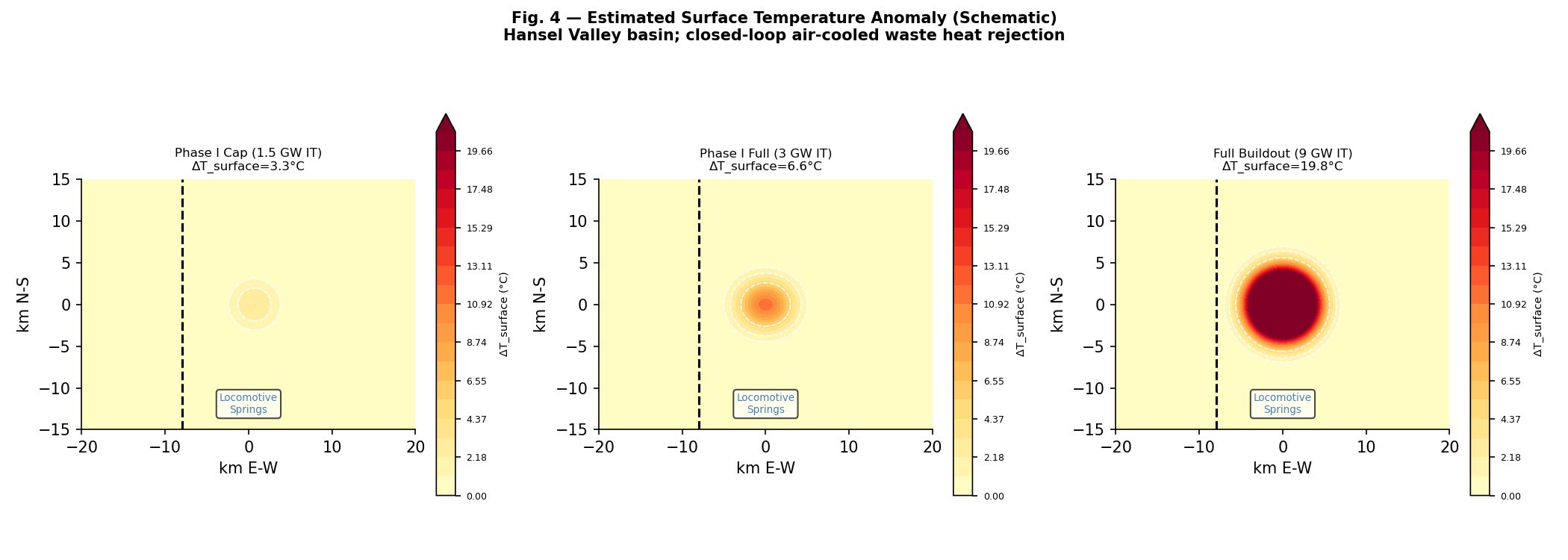
The facility uses closed-loop hydronic cooling with air-cooled dry heat exchangers. All waste heat is rejected to the atmosphere — there is no direct ground heat exchanger. The primary subsurface loading mechanism is the surface temperature anomaly created by the localized heat island. Surface ΔT is computed from an energy balance: ΔT_surface = Q_flux / h_eff where h_eff = 20 W/m²K (composite convection + radiation, desert terrain, average wind 5.6 m/s).
| Scenario | IT Load | Total Thermal | Surface Flux | Surface ΔT |
|---|---|---|---|---|
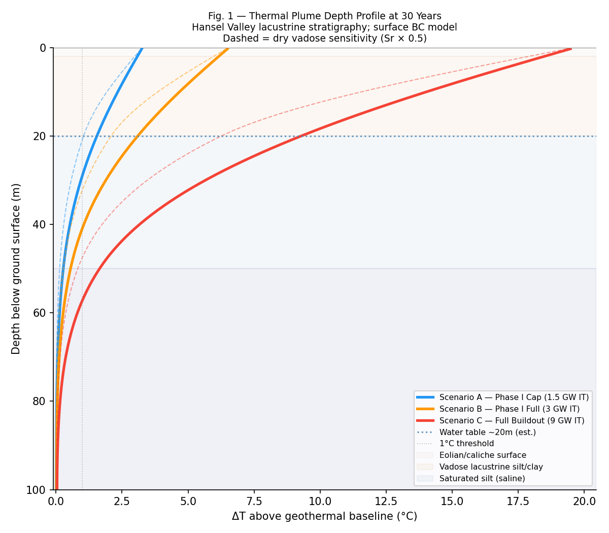
| A — Phase I Cap | 1.5 GW | 2.67 GW | 65.9 W/m² | 3.29°C |
| B — Phase I Full | 3.0 GW | 5.33 GW | 131.8 W/m² | 6.59°C |
| C — Full Buildout | 9.0 GW | 16.0 GW | 395.4 W/m² | 19.77°C |
Area basis: 10,000 acres (40.5 km²) active development footprint. Thermal rejection scales linearly with IT load (16 GW at 9 GW IT per Stratos dossier).
3.2 Scenario A — Phase I Cap (1.5 GW IT)
| Time | ΔT @ 1m | ΔT @ 5m | ΔT @ 10m | ΔT @ 50m | Plume depth (>1°C) |
|---|---|---|---|---|---|
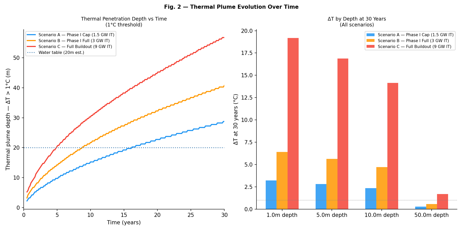
| 1 year | 2.60°C | 0.72°C | 0.06°C | 0.00°C | 3.8 m |
| 10 years | 3.11°C | 2.41°C | 1.64°C | 0.01°C | 15.2 m |
| 30 years | 3.20°C | 2.81°C | 2.36°C | 0.28°C | 28.8 m — past water table |
3.3 Scenario B — Phase I Full (3 GW IT)
| Time | ΔT @ 1m | ΔT @ 5m | ΔT @ 10m | ΔT @ 50m | Plume depth (>1°C) |
|---|---|---|---|---|---|
| 1 year | 5.19°C | 1.43°C | 0.12°C | 0.00°C | 5.2 m |
| 10 years | 6.22°C | 4.81°C | 3.29°C | 0.01°C | 21.8 m — past water table |
| 30 years | 6.40°C | 5.63°C | 4.72°C | 0.56°C | 40.8 m |
3.4 Scenario C — Full Buildout (9 GW IT)
| Time | ΔT @ 1m | ΔT @ 5m | ΔT @ 10m | ΔT @ 50m | Plume depth (>1°C) |
|---|---|---|---|---|---|
| 1 year | 15.57°C | 4.30°C | 0.35°C | 0.00°C | 7.8 m |
| 10 years | 18.67°C | 14.44°C | 9.86°C | 0.04°C | 30.2 m — past water table |
| 30 years | 19.19°C | 16.89°C | 14.15°C | 1.68°C | 56.8 m |
3.5 Peclet Number Analysis — Transport Regime
Pe = (q × ρC_p_fluid × L) / λ_eff, where L = 1 m reference length. For saline lacustrine silts with poor hydraulic connectivity in a flat graben: q_Darcy ≈ 1×10⁻⁸ – 2×10⁻⁷ m/s.
| Darcy Velocity | Pe (vadose, λ=0.43) | Pe (saturated, λ=1.40) | Regime |
|---|---|---|---|
| Low: 1×10⁻⁸ m/s | 0.092 | 0.028 | Conduction dominated |
| Mid: 5×10⁻⁸ m/s | 0.459 | 0.139 | Conduction dominated |
| High: 2×10⁻⁷ m/s | 1.836 | 0.557 | Advection onset (vadose only) |
4. Key Risk Findings
4.1 Thermal Saturation of Hansel Valley Lacustrine Clays
The permanent moisture deficit (MAP 28 cm/yr ≪ PET ~120 cm/yr) means vadose zone conductivity is near dry-state baseline (0.22–0.59 W/m·K at S_r = 0.10–0.25). Heat accumulates in the near-surface rather than dispersing. This is thermal saturation: the soil cannot shed heat fast enough to prevent a growing thermal anomaly that deepens year over year.
The thermal front reaches the water table within 10 years at 3 GW and within 10 years at 9 GW full buildout. By year 30, the plume extends to 56.8 m depth under full buildout conditions — well into the consolidated lakebed formation.
4.2 Soil Dry-Out Feedback Loop
Quantified sensitivity: If S_r drops from 0.20 → 0.10 (plausible under sustained heat loading), λ_eff drops from 0.56 → 0.22 W/m·K — a 61% reduction in conductivity. This would increase thermal penetration depth by approximately 30–50% at the 30-year horizon.
4.3 Locomotive Springs Hydrological Linkage
The Locomotive Springs wetland complex (~15 km south) is a critical migratory bird habitat with regulatory curtailment triggers: if deep groundwater extraction causes a measurable reduction in spring discharge, pumping must be immediately curtailed. Two risk pathways:
4.4 Seismic + Liquefaction Compound Risk
| Scenario | Plume depth 30yr | Sat. zone in plume | Risk |
|---|---|---|---|
| A — Phase I Cap (1.5 GW) | 28.8 m | Yes — 8.8 m into sat. zone | HIGH |
| B — Phase I Full (3 GW) | 40.8 m | Yes — 20.8 m into sat. zone | HIGH |
| C — Full Buildout (9 GW) | 56.8 m | Yes — 36.8 m into sat. zone | HIGH |
The 1934 M6.6 earthquake on the Hansel Valley Fault produced documented liquefaction, sand blows, and lateral spreading across the identical Quaternary lake bed sediments. The fault is <5 km from the facility, near-vertical, with 10–16 ky recurrence. Geothermal warming of the saturated zone reduces effective cohesion in clay-silt mixes by approximately 5–15% per 10°C (Mitchell & Soga, 2005). At full buildout, ΔT in the saturated zone reaches 9.86°C at 10m depth at 10 years. Over a 30–50 year facility lifetime, compound event probability is non-negligible.
5. Substrata vs. Industry Standard Methods
| Dimension | ASHRAE / ASTM Static | Substrata (This Study) |
|---|---|---|
| Thermal conductivity | Single saturated k value | Johansen(S_r) — accounts for dry vadose |
| Moisture coupling | None | Campbell (1985) bucket model |
| Transient penetration | Not computed | 1D layered FD; 1yr, 10yr, 30yr |
| Dry-out feedback | Not considered | Côté & Konrad (2005) Eq. 11 sensitivity |
| Surface BC vs GHX | GHX-centric (IGSHPA) | Surface heat island primary mechanism |
| Heat island estimate | Not in scope | Energy balance; ΔT_surface per scenario |
| Liquefaction compound risk | Not in scope | Analytical screening (gap flagged) |
| Decadal forecast | Not in scope | 1yr, 10yr, 30yr checkpoints |
What static methods miss here: (1) The 2.5–7× overestimate of conductivity from using saturated k on a permanently dry site. (2) The positive feedback between heat loading and moisture depletion in the vadose zone. (3) The decadal timescale of subsurface heat accumulation — static methods show a snapshot, not a trajectory. (4) The compound seismic + thermal risk in the saturated silt zone.
6. Limitations and Confidence Bounds
| Limitation | Impact | What Would Resolve It |
|---|---|---|
| No borehole / TRT data | HIGH | 3–5 TRT boreholes to 50m; confirms λ_eff and water table |
| No SSURGO pull for this site | HIGH | Field moisture sampling + SSURGO API pull |
| Water table depth unknown | HIGH | Water level monitoring wells |
| Atmospheric model absent | HIGH | WRF or mesoscale CFD for basin heat trapping |
| 1D FD vs 3D FV solver | MEDIUM | Run full 3D FV (thermal-advection-diffusion.ts) |
| Geothermal gradient estimate | MEDIUM | Heat flow measurements to 200m depth |
| No fault distance measurement | MEDIUM | LiDAR fault mapping + site survey |
| Saline pore fluid ρC_p | LOW | Lab measurement of formation water |
Surface ΔT estimates: MEDIUM — energy balance correct; h_eff ±30%.
Depth penetration profile: MEDIUM — 1D approximation; 3D would be warmer near cluster cores.
Locomotive Springs linkage: LOW — no groundwater flow model.
Liquefaction risk: QUALITATIVE ONLY — no SPT-N, no seismic hazard attenuation model.